Site-Specific PUSCH Autoencoder
Overview
This demo implements an end-to-end autoencoder for the 5G NR Physical Uplink Shared Channel (PUSCH), by jointly optimizing a trainable constellation at the transmitter and a neural MIMO detector at the receiver [1]. The system operates over site-specific ray-traced channels derived from a realistic Munich urban environment, enabling the autoencoder to adapt to the propagation characteristics of this specific deployment.
The autoencoder applies concepts from classical communication autoencoders (O’Shea & Hoydis, 2017) to a multi-user MIMO uplink scenario with 4 UEs (each with 4 antennas) transmitting to a base station with 32 antennas. This demo builds upon the following Sionna tutorials:
System Architecture
The PUSCH link (PUSCHLinkE2E) implements a complete uplink chain.
The architecture diagram depicting this class is shown below.


For details regarding the OFDM slot structure, the MIMO configuration, and the 5G NR PUSCH parameters used in this demo, see the code-snippet extracted from Config below.
    # =========================================================================
    # User-Configurable Parameters
    # =========================================================================
    # Number of BS antennas (cross-polarized). Default 32 provides sufficient
    # spatial DoF to separate 4 single-layer UE streams with reasonable margin.
    # Must be even since the antenna array uses cross-polarization.
    num_bs_ant: int = 32

    # =========================================================================
    # OFDM / Slot Structure
    # =========================================================================
    # Subcarrier spacing determines the slot duration and Doppler tolerance.
    # 30 kHz is standard for FR1 (sub-6 GHz) NR deployments.
    _subcarrier_spacing: float = field(init=False, default=30e3, repr=False)

    # 14 OFDM symbols per slot is the standard NR slot structure with
    # normal cyclic prefix. This must match the CIR time-domain sampling.
    _num_time_steps: int = field(init=False, default=14, repr=False)

    # =========================================================================
    # MIMO Configuration
    # =========================================================================
    # 4 UEs enables meaningful MU-MIMO interference while keeping
    # computational complexity manageable for the purpose of this demo.
    _num_ue: int = field(init=False, default=4, repr=False)

    # Single base station - multi-cell scenarios not currently supported.
    _num_bs: int = field(init=False, default=1, repr=False)

    # 4 UE antennas (2x2 cross-polarized) matches typical smartphone designs
    # and enables spatial multiplexing on the uplink.
    _num_ue_ant: int = field(init=False, default=4, repr=False)

    # =========================================================================
    # PUSCH / 5G NR Physical Layer Parameters
    # =========================================================================
    # 16 PRBs = 192 subcarriers, suitable for moderate throughput scenario.
    _num_prb: int = field(init=False, default=16, repr=False)

    # MCS index 14 with table 1 yields 16-QAM with ~0.6 coderate,
    # providing a good balance between spectral efficiency and robustness.
    _mcs_index: int = field(init=False, default=14, repr=False)

    # Single layer per UE simplifies the autoencoder while still enabling
    # meaningful MU-MIMO scenarios with 4 co-scheduled UEs.
    _num_layers: int = field(init=False, default=1, repr=False)

    # MCS table 1 is the default for PUSCH without 256-QAM support.
    _mcs_table: int = field(init=False, default=1, repr=False)

    # Frequency-domain processing avoids OFDM modulation/demodulation
    # overhead and simplifies the neural network input structure.
    _domain: str = field(init=False, default="freq", repr=False)

    # Derived from MCS tables in __post_init__. Not set at field definition
    # since they require MCSDecoderNR computation.
    _num_bits_per_symbol: int = field(init=False, repr=False)
    _target_coderate: float = field(init=False, repr=False)
Trainable Transmitter
The transmitter (PUSCHTrainableTransmitter) subclasses Sionna’s PUSCHTransmitter with learnable constellation points. A random set of 4 (in the case of 16-QAM) constellation points are initialized with positive real and imaginary components. They were further constrained so that neither the real nor the imaginary components can be zero-valued, nor is origin allowed to be a constellation point. The points so chosen are then reflected across the I-axis, the Q-axis, and the origin to generate a symmetric constellation. A representative diagram is shown below.


The steps involved in setting up the custom constellation are shown in the code-snippet below (extracted from PUSCHTrainableTransmitter).
    def _setup_custom_constellation(self):
        """
        Initialize symmetric trainable constellation and learnable labeling.

        For 16-QAM (num_bits_per_symbol=4):
        - Stores 4 base points in Q1 as trainable variables
        - Other 12 points computed via reflections (enforces symmetry)
        - Labeling initialized to identity matrix (preserves structure initially)

        Notes
        -----
        Even with symmetric geometry, we preserve flexible labeling to allow
        the optimizer to discover optimal bit-to-symbol assignments that may
        differ from standard Gray coding.
        """
        num_points = 2**self._num_bits_per_symbol
        self._num_constellation_points = num_points
        self._num_base_points = num_points // 4

        if self._training:
            # Training mode: Use symmetric random initialization
            constellation_points = self.generate_random_symmetric_constellation(
                num_points, seed=None  # No seed = different init each run
            )
            # Extract just the base points (Q1 only)
            base_points = constellation_points[: self._num_base_points]
        else:
            # Inference mode: Use standard QAM as placeholder
            constellation_points = Constellation(
                "qam", num_bits_per_symbol=self._num_bits_per_symbol
            ).points
            # For QAM, assume first quarter are Q1 points (this is approximate)
            base_points = constellation_points[: self._num_base_points]

        # Store ONLY base points as trainable variables
        init_r = tf.math.real(base_points)
        init_i = tf.math.imag(base_points)

        self._base_points_r = tf.Variable(
            tf.cast(init_r, self.rdtype),
            trainable=self._training,
            name="constellation_base_real",
        )
        self._base_points_i = tf.Variable(
            tf.cast(init_i, self.rdtype),
            trainable=self._training,
            name="constellation_base_imag",
        )

        # Initialize labeling logits to identity-like matrix
        # This means bit pattern i initially maps to constellation point i
        identity_scale = 5.0  # Start sharply peaked at identity
        init_logits = tf.eye(num_points) * identity_scale

        self._labeling_logits = tf.Variable(
            tf.cast(init_logits, self.rdtype),
            trainable=self._training,
            name="labeling_logits",
        )

        # Create constellation object for compatibility with Sionna internals
        # (used by resource grid mapper, etc.)
        # Initialize with full reflected constellation
        full_constellation = self.get_normalized_constellation()
        self._constellation = Constellation(
            "custom",
            num_bits_per_symbol=self._num_bits_per_symbol,
            points=full_constellation,
            normalize=False,
            center=False,
        )
The remaining operations are as in Sionna’s PUSCHTransmitter. First, information bits are encoded into a transport block, which are then mapped to QAM constellation symbols by the Mapper. The constellation points are initialized to 16-QAM points. They are set to be trainable when the autoencoder is being designed, and non-trainable when evaluating the baseline scenarios. Next, the modulated symbols are split into different layers which are then mapped onto OFDM resource grids. If precoding is enabled, the resource grids are further precoded so that there is one for each transmitter and antenna port, and these are the outputs of the transmit chain.
Trainable Receiver
The receiver implements a hybrid classical/neural-network architecture. The sequence of operations implemented are as follows. First, channel estimation is performed. If channel_estimator is chosen to be “perfect”, this step is skipped and the perfect channel state information (CSI) is used downstream. Next, MIMO detection is carried out with an LMMSE Detector. The resulting LLRs for each layer are then combined to transport blocks and are decoded.
The only modification in the subclassed trainable receiver (PUSCHTrainableReceiver) is the provision to choose between a classical LMMSE detector versus the neural-network based detector:
        # =====================================================================
        # MIMO Detection with Constellation Synchronization
        # =====================================================================
        # Pass trainable constellation to ensure demapper uses same points as mapper.
        # This is critical for correct gradient computation in autoencoder training.
        constellation = self._get_normalized_constellation()
        if constellation is not None:
            llr = self._mimo_detector(
                y, h_hat, err_var, no, constellation=constellation
            )
        else:
            llr = self._mimo_detector(y, h_hat, err_var, no)
Neural Detector
The neural detector (PUSCHNeuralDetector) implements a residual learning architecture that refines LS channel estimates and LMMSE soft symbols rather than learning detection from scratch. The motivation behind this design is that learning residual corrections to classical estimates is more stable than learning detection from scratch. The architecture (see diagram below) processes shared features through convolutional residual blocks to obtain channel estimation refinement before proceeding to refine LLR through MIMO-OFDM detection head. Note that while the conventional LS channel estimation relies exclusively on the pilot symbols, the channel estimation refinement additionally utilizes data symbols also.


Three trainable correction scales control how much the neural network deviates from classical LS channel estimation followed by LMMSE MIMO-OFDM detection. These scales start at zero (pure classical behavior) and are learned during training, providing interpretable indicators of where neural refinement helps most.
The initialization of various components in the shared backbone, the channel estimation refinement head, and the MIMO-OFDM detection head are as shown below:
        # =====================================================================
        # Shared Backbone Network
        # =====================================================================
        # Processes all input features to learn representations useful for both
        # channel estimation refinement and detection. Sharing weights between
        # these tasks acts as implicit regularization and reduces parameters.
        self._shared_conv_in = Conv2D(
            filters=self.num_conv2d_filters,
            kernel_size=(3, 3),
            padding="same",
            name="shared_conv_in",
        )
        self._shared_res_blocks = [
            Conv2DResBlock(
                filters=self.num_conv2d_filters,
                kernel_size=self.kernel_size,
                name=f"shared_resblock_{i}",
            )
            for i in range(self.num_shared_res_blocks)
        ]

        # =====================================================================
        # Channel Estimation Refinement Head
        # =====================================================================
        # Lightweight head that projects shared features to channel corrections.
        # Separate outputs for Δh (complex) and Δlog(err_var) (real).
        self._ce_head_conv1 = tf.keras.Sequential(
            [
                Conv2D(self.num_conv2d_filters, (3, 3), padding="same"),
                LayerNormalization(axis=-1),
                tf.keras.layers.LeakyReLU(0.1),
                Conv2D(self.num_conv2d_filters, (3, 3), padding="same"),
                LayerNormalization(axis=-1),
                tf.keras.layers.LeakyReLU(0.1),
            ],
            name="ce_head_conv1",
        )

        # Output layer for channel correction: 2 * Nr * S values (real + imag)
        self._ce_head_out_h = Conv2D(
            filters=2 * Nr * S,
            kernel_size=(1, 1),
            padding="same",
            activation=None,
            name="ce_head_out_h",
        )

        # Output layer for error variance log-correction: S values per RE
        self._ce_head_out_loge = Conv2D(
            filters=S,
            kernel_size=(1, 1),
            padding="same",
            activation=None,
            name="ce_head_out_loge",
        )

        # =====================================================================
        # Detection Continuation Network
        # =====================================================================
        # After LMMSE equalization with refined estimates, this network learns
        # to correct the resulting LLRs based on both the original features
        # and the LMMSE outputs (symbol estimates, effective noise).
        self._c_lmmse_feats = (
            2 * S  # x_lmmse: equalized symbols (real + imag)
            + S  # no_eff: post-equalization noise variance (log scale)
            + S * self._num_bits_per_symbol  # llr_lmmse: baseline soft bits
        )

        # Injection convolution fuses shared backbone features with LMMSE outputs
        self._det_inject_conv = Conv2D(
            filters=self.num_conv2d_filters,
            kernel_size=(3, 3),
            padding="same",
            name="det_inject_conv",
        )

        # Additional ResBlocks for LLR refinement
        self._det_res_blocks = [
            Conv2DResBlock(
                filters=self.num_conv2d_filters,
                kernel_size=self.kernel_size,
                name=f"det_resblock_{i}",
            )
            for i in range(self.num_det_res_blocks)
        ]

        # Output convolution produces LLR corrections for all bits
        self._det_conv_out = Conv2D(
            filters=S * self._num_bits_per_symbol,
            kernel_size=(3, 3),
            padding="same",
            activation=None,
            name="det_conv_out",
        )

        # =====================================================================
        # Trainable Correction Scales
        # =====================================================================
        # Initialize all scales to 0.0 so that initial output matches classical
        # LMMSE exactly. This provides a stable starting point and enables
        # graceful degradation if training fails to improve on classical.

        # Channel estimate correction: h_refined = h_ls + scale * delta_h
        # Unbounded since corrections can be positive or negative.
        self._h_correction_scale = tf.Variable(
            0.0, trainable=True, name="h_correction_scale", dtype=tf.float32
        )

        # LLR correction: llr_final = llr_lmmse + scale * delta_llr
        # Unbounded to allow both confidence increase and decrease.
        self._llr_correction_scale = tf.Variable(
            0.0, trainable=True, name="llr_correction_scale", dtype=tf.float32
        )

        # Error variance correction in log domain for numerical stability:
        # err_var_refined = exp(log(err_var) + scale * delta_log_err)
        # Uses softplus(raw_value) to ensure positivity; softplus(0) = ln(2) ≈ 0.69
        # but we want initial scale ≈ 1.0, and softplus(0.54) ≈ 1.0
        # For simplicity, initialize to 0.0; the network will adapt.
        self._err_var_correction_scale_raw = tf.Variable(
            0.0, trainable=True, name="err_var_correction_scale_raw", dtype=tf.float32
        )
The features are processed by the shared backbone network as shown below:
        # =====================================================================
        # Shared Backbone Forward Pass
        # =====================================================================
        shared_features = self._shared_conv_in(shared_input)
        for block in self._shared_res_blocks:
            shared_features = block(shared_features)
        # shared_features: [B, H, W, num_filters]
by the channel estimation head as shown below:
        # =====================================================================
        # Channel Estimation Refinement Head
        # =====================================================================
        ce_hidden = self._ce_head_conv1(shared_features)

        delta_h_raw = self._ce_head_out_h(ce_hidden)  # [B,H,W, 2*Nr*S]
        delta_loge = self._ce_head_out_loge(ce_hidden)  # [B,H,W, S]

        # Parse channel correction into complex format
        delta_h_raw = tf.cast(delta_h_raw, tf.float32)
        delta_h_r = delta_h_raw[..., : Nr * S]
        delta_h_i = delta_h_raw[..., Nr * S :]
        delta_h_c = tf.complex(delta_h_r, delta_h_i)
        delta_h_c = tf.reshape(delta_h_c, [B, H, W, Nr, S])

        # =====================================================================
        # Apply Scaled Channel Refinement
        # =====================================================================
        # Additive correction: h_refined = h_ls + scale * delta_h
        # Scale starts at 0, so initial behavior matches LS exactly.
        h_scale = tf.cast(self._h_correction_scale, tf.complex64)
        h_flat_refined = h_flat + h_scale * tf.cast(delta_h_c, h_flat.dtype)

        # =====================================================================
        # Apply Scaled Error Variance Refinement (Log Domain)
        # =====================================================================
        # Multiplicative correction in log domain for numerical stability:
        # err_var_refined = exp(log(err_var) + scale * delta_log_err)
        # This ensures err_var remains positive regardless of delta magnitude.
        err_var_scale = self.err_var_correction_scale  # softplus-transformed
        log_err = tf.math.log(err_var_flat + 1e-10)
        log_err_refined = log_err + err_var_scale * tf.cast(delta_loge, log_err.dtype)
        err_var_flat_refined = tf.exp(log_err_refined)
and by the MIMO-OFDM detection head as shown below:
        # Injection convolution reduces dimensions and fuses information
        det_features = self._det_inject_conv(combined_features)

        # Additional ResBlocks for LLR refinement
        for block in self._det_res_blocks:
            det_features = block(det_features)

        # Predict LLR corrections
        llr_correction = self._det_conv_out(det_features)
The residual blocks follow the standard design which consists of cascaded units of layer normalization, activation function, and convolutional layer, with a skip connection to avoid gradient vanishing.


Ray-traced Channel
Sionna-RT module can be used simulate environment-specific and physically accurate channel realizations for a given scene and user position. It is built on top of Mitsuba 3.
Setting up the ray tracer
The ray-traced channel generated using Sionna-RT consists of a single-cell, multiuser MIMO layout with one base station serving four users, equipped with 32 antennas and 4 antennas, respectively, using planar arrays with half-wavelength element spacing and cross polarization. An integrated urban scene located in Munich is loaded and the base station is placed at [8.5, 21, 27], with its orientation fixed toward the service area, while a static camera at [0, 80, 500] is used to generate verification renders. Propagation is computed deterministically with a maximum interaction depth of 5, spatial resolution cell size of (1.0, 1.0), and samples per transmitter set to 10000, producing a dense radio map of path gain across the environment. For more details see the code-snippet extracted from Config below.
    # =========================================================================
    # Ray-Tracing Path Solver Configuration
    # =========================================================================
    # Maximum reflection depth. 5 captures dominant multipath while
    # avoiding excessive computation from high-order reflections.
    _max_depth: int = field(init=False, default=5, repr=False)

    # Path gain thresholds for UE position sampling. Positions with path
    # gain outside [-130, 0] dB are excluded to avoid dead zones and
    # unrealistic near-field scenarios.
    _min_gain_db: float = field(init=False, default=-130.0, repr=False)
    _max_gain_db: float = field(init=False, default=0.0, repr=False)

    # Sampling annulus distances from BS. Inner radius (5m) avoids
    # near-field effects; outer radius (400m) covers typical urban cell.
    _min_dist_m: float = field(init=False, default=5.0, repr=False)
    _max_dist_m: float = field(init=False, default=400.0, repr=False)

    # =========================================================================
    # Radio Map Visualization Parameters
    # =========================================================================
    # Cell size for radio map discretization (meters). 1m provides
    # sufficient resolution for urban canyon visualization.
    _rm_cell_size: Tuple[float, float] = field(
        init=False, default=(1.0, 1.0), repr=False
    )

    # Monte Carlo samples per TX for radio map computation. 10^7 samples
    # provides smooth coverage maps with low variance.
    _rm_samples_per_tx: int = field(init=False, default=10**7, repr=False)

    # Visualization thresholds. -110 dBm floor matches typical UE sensitivity;
    # clip_at=12 prevents outliers from dominating the colormap.
    _rm_vmin_db: float = field(init=False, default=-110.0, repr=False)
    _rm_clip_at: float = field(init=False, default=12.0, repr=False)

    # Output image resolution (width, height) in pixels.
    _rm_resolution: Tuple[int, int] = field(init=False, default=(650, 500), repr=False)

    # Samples per pixel for anti-aliased rendering.
    _rm_num_samples: int = field(init=False, default=4096, repr=False)
The rendered figure below visualizes this radio map overlaid on the scene geometry, and shows the transmitter placement, the dominant propagation regions, and the obstruction effects prior to receiver sampling. Although the focus is geometric, the physical-layer context is fixed via a subcarrier spacing of 30 kHz and num_time_steps = 14, which later determine the temporal resolution of the channel representation.
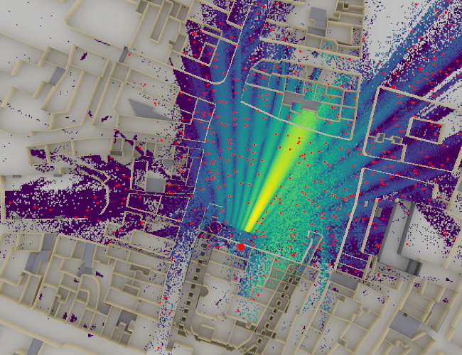
Ray-traced Munich urban scene showing sampled UE positions for CIR generation.
Creating a CIR dataset
Receiver positions are sampled in batches of 500 from the radio map using path-gain constraints (-130 dB to 0 dB) and a distance window of 5-400 m around the base station, ensuring physically meaningful links. For each batch, all receivers are updated in the scene and multipath propagation is recomputed with up to 10000 paths per transmitter, preserving line-of-sight and higher-order interactions up to the specified depth. Continuous path delays and complex gains are then discretized into channel impulse responses using a sampling frequency equal to the subcarrier spacing (30 kHz) over 14 time steps, after which all CIRs are padded to a common maximum number of paths and concatenated. The resulting tensors yield a geometry-consistent CIR dataset that can be repeatedly sampled during training and inference in fixed-size batches (e.g., batch_size = 20) for link-level simulations while preserving the underlying ray-traced propagation structure. For more details, see CIRManager.
Training and Results
With the prerequisite step of generating CIR data via the CIRManager accomplished, the autoencoder can be trained to minimize binary cross-entropy (BCE) loss between predicted LLRs and transmitted coded bits. The system uses gradient accumulation over 16 micro-batches with separate Adam optimizers for transmitter variables (learning rate of 1e-2), receiver correction scales (learning rate of 1e-2), and neural network weights (learning rate of 1e-4), all with cosine decay schedules over 5000 iterations. The important pieces in the training logic are shown below:
# =============================================================================
# Gradient Computation Functions
# =============================================================================
# Gradient accumulation: 16 micro-batches averaged to reduce variance
# This simulates larger batch training without memory overhead
accumulation_steps = 16


@tf.function
def compute_grads_single():
    """
    Compute gradients for a single random SNR micro-batch.

    Returns
    -------
    loss : tf.Tensor
        BCE loss for this micro-batch.
    grads : list of tf.Tensor
        Gradients for all trainable variables.
    """
    ebno_db = tf.random.uniform(
        [training_batch_size], minval=ebno_db_min, maxval=ebno_db_max
    )
    with tf.GradientTape() as tape:
        loss = model(training_batch_size, ebno_db)
    grads = tape.gradient(loss, all_vars)
    return loss, grads


def compute_accumulated_grads():
    """
    Compute gradients accumulated over multiple micro-batches.

    Averages gradients from accumulation_steps forward passes to reduce
    variance. This simulates larger batch training without memory overhead.

    Returns
    -------
    avg_loss : tf.Tensor
        Mean BCE loss over all micro-batches.
    grads_tx : list of tf.Tensor
        Averaged gradients for transmitter variables.
    grads_scales : list of tf.Tensor
        Averaged gradients for correction scale variables.
    grads_rx_nn : list of tf.Tensor
        Averaged gradients for neural network weight variables.
    """
    accumulated_grads = [tf.zeros_like(v) for v in all_vars]
    total_loss = 0.0

    for _ in range(accumulation_steps):
        loss, grads = compute_grads_single()
        accumulated_grads = [ag + g for ag, g in zip(accumulated_grads, grads)]
        total_loss += loss

    # Average over accumulation steps
    accumulated_grads = [g / accumulation_steps for g in accumulated_grads]
    avg_loss = total_loss / accumulation_steps

    # Split into variable groups for separate optimizer application
    grads_tx = accumulated_grads[:n_tx]
    grads_scales = accumulated_grads[n_tx : n_tx + n_scales]
    grads_rx_nn = accumulated_grads[n_tx + n_scales :]

    return avg_loss, grads_tx, grads_scales, grads_rx_nn


# =============================================================================
# Main Training Loop
# =============================================================================
loss_history = []

# Suffix for all output files
ant_suffix = f"_ant{num_bs_ant}"

print(f"Starting training for {num_training_iterations} iterations...")
print("  TX LR: 1e-2, RX Scales LR: 1e-2, RX NN LR: 1e-4")
print(f"  Output files will have suffix: {ant_suffix}")

for i in range(num_training_iterations):
    avg_loss, grads_tx, grads_scales, grads_rx_nn = compute_accumulated_grads()
    loss_value = float(avg_loss.numpy())
    loss_history.append(loss_value)

    # Simultaneous update: all variable groups updated together
    optimizer_tx.apply_gradients(zip(grads_tx, tx_vars))
    optimizer_scales.apply_gradients(zip(grads_scales, rx_scale_vars))
    optimizer_rx.apply_gradients(zip(grads_rx_nn, nn_rx_vars))

    # Progress display (overwrite same line)
    print(
        "Iteration {}/{}  BCE: {:.4f}".format(
            i + 1, num_training_iterations, loss_value
        ),
        end="\r",
        flush=True,
    )

    # Periodic checkpointing to resume from crashes
    if (i + 1) % 1000 == 0:
        os.makedirs(os.path.join(DEMO_DIR, "results"), exist_ok=True)
        save_path = os.path.join(
            DEMO_DIR, "results", f"PUSCH_autoencoder_weights_iter_{i + 1}{ant_suffix}"
        )

        # Store both raw variables and normalized constellation
        normalized_const = (
            model._pusch_transmitter.get_normalized_constellation().numpy()
        )
        weights_dict = {
            "tx_weights": [
                v.numpy() for v in model._pusch_transmitter.trainable_variables
            ],
            "rx_weights": [
                v.numpy() for v in model._pusch_receiver.trainable_variables
            ],
            "tx_names": [v.name for v in model._pusch_transmitter.trainable_variables],
            "rx_names": [v.name for v in model._pusch_receiver.trainable_variables],
            "normalized_constellation": normalized_const,
        }
        with open(save_path, "wb") as f:
            pickle.dump(weights_dict, f)
        print(f"\n[Checkpoint] Saved weights at iteration {i + 1} -> {save_path}")
Eb/N0 is sampled uniformly from -2 to 9 dB for each batch for the baseline design and from -1 dB to 2 dB for the end-to-end autoencoder design, enabling the autoencoder to learn a robust parameter set across the chosen operating SNR range. Performance is evaluated using BER and BLER Monte Carlo simulation, comparing the trained autoencoder against baseline LMMSE detection with both perfect and imperfect (LS-estimated) CSI.
As shown in the inset diagram in the two plots below, for the baseline deseign, the performance gap is wider at low SNR between perfect CSI case and least-squares CSI case. Furthermore, given that a custom non-uniform constellation optimized for a narrower Eb/N0 range assumes a markedly different shape compared to another that is optimized for a wider range [2], the Eb/N0 range of -1 dB to 2 dB was selected to train the constellation of the end-to-end autoencoder design.
The main (non-inset) plot for both BER and BLER reveals that the trainable constellation along with the neural detector substantially improves the performance compared to the baseline case.
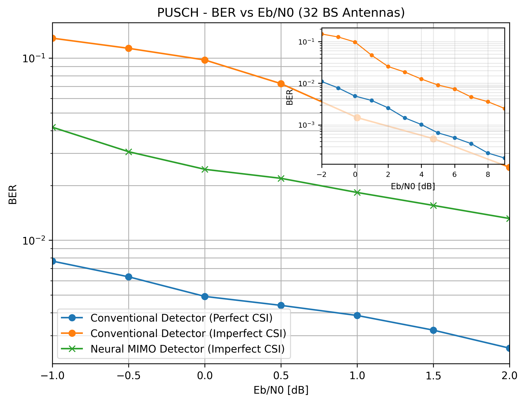
BER comparison: autoencoder vs. baseline LMMSE with 32 BS antennas.
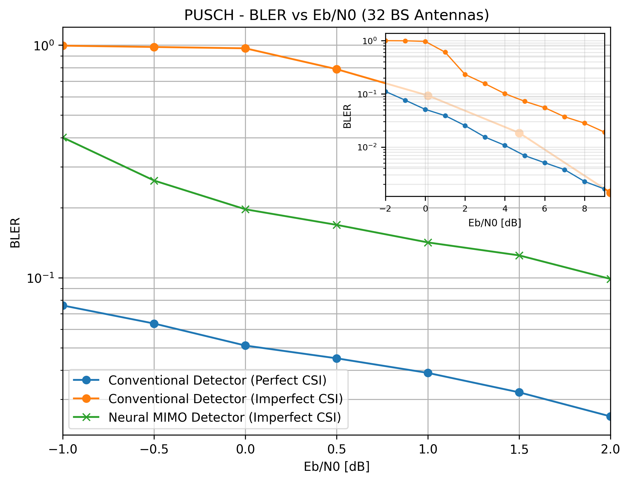
BLER comparison: autoencoder vs. baseline LMMSE with 32 BS antennas.
The learned constellation for this scenario is shown below.
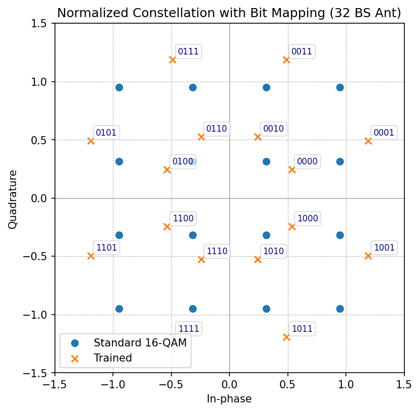
Learned constellation geometry (32 BS antennas) compared to standard 16-QAM.
The learned constellation points reveal that they adapt to the site-specific channel statistics while maintaining sufficient minimum distance for reliable detection. The autoencoder does not yet match the perfect-CSI baseline, indicating room for increased model capacity, architectural refinements, hyperparameter optimization, or alternative training strategies.
References
[1] T. O’Shea and J. Hoydis, “An Introduction to Deep Learning for the Physical Layer,” in IEEE Transactions on Cognitive Communications and Networking, vol. 3, no. 4, pp. 563-575, Dec. 2017, doi: 10.1109/TCCN.2017.2758370.
[2] Manuel Fuentes Muela, “Non-Uniform Constellations for Next-Generation Digital Terrestrial Broadcast Systems.” (2017).