Digital Predistortion (DPD)
Overview
This demo implements digital pre-distortion (DPD) for power amplifier (PA) linearization in 5G-like OFDM wireless systems. In this demo, the use of Sionna’s API is limited only to generate the transmit signal used in DPD design. The subsequent demos utilize Sionna’s features more extensively.
Power amplifiers are well-known to be inherently nonlinear devices that introduce amplitude-dependent gain compression (AM/AM) and phase distortion (AM/PM), along with memory effects from thermal and electrical time constants. These nonlinearities cause spectral regrowth that violates adjacent channel leakage ratio (ACLR) specifications and in-band distortion that degrades error vector magnitude (EVM). Mitigating these effects is important in order to meet spectral emission mask requirements set by regulatory bodies such as the Federal Communications Commission (FCC).
DPD compensates for PA nonlinearity by applying a pre-inverse transformation to the input signal such that the PA output becomes approximately linear. The demo implements two DPD approaches, namely Least-Squares (LS) DPD using the Memory Polynomial model [1] and Neural Network (NN) DPD [2] using a feedforward residual architecture, both trained via the indirect learning architecture (ILA).
System Architecture
The DPD system operates on a single-user OFDM transmitter with 16-QAM modulation, rate-1/2 LDPC coding, and 624 active subcarriers across a 1024-point FFT with 15 kHz spacing. The baseband signal at 15.36 MHz is upsampled to the PA operating rate of 122.88 MHz (8x oversampling) using an interpolator before predistortion and PA modeling. For more details, see the code-snippet extracted from Config below.
    # --- Mutable parameters (user-configurable at initialization) ---
    seed: int = field(default=42)
    batch_size: int = field(default=100)

    # --- System parameters (immutable) ---
    # Single-user SISO configuration
    _num_ut: int = field(init=False, default=1, repr=False)
    _num_ut_ant: int = field(init=False, default=1, repr=False)
    _num_streams_per_tx: int = field(init=False, default=1, repr=False)

    # --- Resource grid parameters (immutable) ---
    _num_ofdm_symbols: int = field(init=False, default=8, repr=False)
    _fft_size: int = field(init=False, default=1024, repr=False)
    _subcarrier_spacing: float = field(init=False, default=15000.0, repr=False)
    _num_guard_carriers: Tuple[int, int] = field(init=False, repr=False)
    _dc_null: bool = field(init=False, default=True, repr=False)
    _cyclic_prefix_length: int = field(init=False, default=72, repr=False)
    _pilot_pattern: str = field(init=False, default="kronecker", repr=False)
    _pilot_ofdm_symbol_indices: List[int] = field(init=False, repr=False)

    # --- Modulation and coding parameters (immutable) ---
    _num_bits_per_symbol: int = field(init=False, default=4, repr=False)
    _coderate: float = field(init=False, default=0.5, repr=False)
PA Model
The PA (PowerAmplifier) is modeled as a 7th-order Memory Polynomial with 4 memory taps, characterized from a WARP v3 board. The model captures both static nonlinearity and short-term memory effects using the equation:
Indirect Learning Architecture
The indirect learning architecture (see diagram below) operates by exploiting the relationship between the desired PA output, the actual PA output, and the original input signal. During training, the post-distorter is learned first by mapping the PA output back to the pre-distorter output. The pre-distorter is then updated using these learned parameters, thereby driving the error toward zero. At convergence, the cascade of the pre-distorter and the PA behaves as a (nearly) linear system, with the signals at the inputs of the pre-distorter and post-distorter being identical. As a consequence, both blocks produce the same output and the resulting error signal vanishes.


The code snippet below from _training_forward() of NN_DPDSystem implements the architecture diagram described for NN-DPD. The corresponding implementation for LS-DPD is similar (see _ls_training_iteration() of LS_DPDSystem).
        # Steps 1-3: Forward through predistorter and PA.
        signals = self._forward_signal_path(x)
        u_norm = signals["u_norm"]
        y_comp = signals["y_comp"]

        # Target is predistorter output (gradient stopped).
        # The goal is to match postdistorter and predistorter outputs.
        u_target = tf.stop_gradient(u_norm)

        # Normalize PA output for postdistorter input.
        y_norm, _ = self._normalize_to_unit_power(y_comp)

        # Step 4: Apply postdistorter (this path receives gradients).
        u_hat_norm = self._dpd(y_norm, training=True)

        # Step 5: Compute MSE loss on real/imag components.
        # Split complex into [real, imag] for standard MSE computation.
        u_target_ri = tf.stack(
            [tf.math.real(u_target), tf.math.imag(u_target)], axis=-1
        )
        u_hat_ri = tf.stack(
            [tf.math.real(u_hat_norm), tf.math.imag(u_hat_norm)], axis=-1
        )

        loss = self._loss_fn(u_target_ri, u_hat_ri) * self._loss_scale
Least-Squares DPD
The LS-DPD (LeastSquaresDPD) uses the same Memory Polynomial structure as the PA model. Coefficients are computed via closed-form least-squares estimation with regularization. The ILA trains a postdistorter on the gain-normalized PA output, then copies these coefficients to the pre-distorter.
    def _ls_estimation(self, X, y):
        """
        Compute least-squares coefficient estimate.

        Solves the regularized least-squares problem:
        ``min ||X @ coeffs - y||^2 + lambda*||coeffs||^2``

        Parameters
        ----------
        X : tf.Tensor
            Basis matrix, shape ``[num_samples, n_coeffs]``.
        y : tf.Tensor
            Target signal, shape ``[num_samples]``.

        Returns
        -------
        tf.Tensor
            Estimated coefficients, shape ``[n_coeffs, 1]``.

        Notes
        -----
        The first (memory_depth + lag_depth - 1) and last lag_depth samples
        are excluded from the fit to avoid edge effects from the delay
        operations in the basis matrix construction.

        L2 regularization (lambda=1e-3) prevents ill-conditioning when the
        basis matrix has near-collinear columns.
        """
        # Exclude edge samples affected by delays.
        start = self._memory_depth + self._lag_depth - 1
        end = -self._lag_depth if self._lag_depth > 0 else None
        X_slice, y_slice = X[start:end], tf.reshape(y[start:end], [-1, 1])

        # Regularized least-squares via TensorFlow's lstsq.
        return tf.linalg.lstsq(X_slice, y_slice, l2_regularizer=1e-3)
Neural Network DPD
The NN-DPD (NeuralNetworkDPD) uses a feedforward architecture (see diagram below).


This network processes sliding windows of complex samples (split into real/imaginary channels), and their envelopes raised to powers of 2, 4, and 6 through residual blocks encapsulated between input and output dense layers. The residual blocks follow the standard design which consists of cascaded units of layer normalization, activation function, and dense layer, with a skip connection to avoid gradient vanishing. The output layer is initialized to zeros, ensuring the initial network output equals the input (identity function via skip connection). This provides a stable starting point where training learns corrections relative to the pass-through behavior.
The input/output dense layers and the residual blocks are initialized as shown below:
        # Project input features to hidden dimension.
        self._input_dense = Dense(
            self._num_filters,
            activation=None,
            kernel_initializer="glorot_uniform",
            name="input_projection",
        )

        # Stack of residual blocks for deep nonlinear processing.
        self._res_blocks = [
            ResidualBlock(
                units=self._num_filters,
                num_layers=self._num_layers_per_block,
            )
            for _ in range(self._num_res_blocks)
        ]

        # Output projection: hidden -> [real, imag].
        # Zero initialization ensures initial output is identity (via skip).
        self._output_dense = Dense(
            2,
            activation=None,
            kernel_initializer="zeros",
            bias_initializer="zeros",
            name="output",
        )
and the features are processed as shown below:
        # Forward through network.
        z = self._input_dense(features)  # [B, N, num_filters]

        for block in self._res_blocks:
            z = block(z)

        z = self._output_dense(z)  # [B, N, 2]

        # Skip connection: network learns correction relative to identity.
        z = z + skip
Training
Both DPD methods are trained using the ILA as described previously. To recap, an overview of the procedure followed is:
Generate OFDM signal and upsample to PA rate
Apply pre-distorter: \(u = \text{DPD}(x)\)
Pass through PA: \(y = \text{PA}(u)\)
Normalize by PA gain: \(y_{\text{norm}} = y / G\)
Compute loss: \(\mathcal{L} = \|\text{DPD}(y_{\text{norm}}) - u\|^2\)
Update DPD parameters
LS-DPD converges in 3-5 iterations using Newton-style updates with learning rate 0.75.
NN-DPD was trained over 25000 gradient descent iterations with Adam optimizer (learning rate 1e-3). Gradient accumulation over 4 mini-batches of size 16 (for an effective batch size of 64) was implemented as follows:
for i in range(start_iteration, target_iteration):
    # Forward pass and gradient computation.
    loss, grads = train_step(batch_size_tensor)

    # Accumulate gradients.
    for acc_g, g in zip(accumulated_grads, grads):
        acc_g.assign_add(g)

    # Apply accumulated gradients every ACCUMULATION_STEPS.
    if (i + 1) % ACCUMULATION_STEPS == 0:
        # Average gradients over accumulation window.
        avg_grads = [g / ACCUMULATION_STEPS for g in accumulated_grads]
        optimizer.apply_gradients(zip(avg_grads, system.trainable_variables))
        # Reset accumulators for next window.
        for acc_g in accumulated_grads:
            acc_g.assign(tf.zeros_like(acc_g))

    loss_value = float(loss.numpy())
    loss_history.append(loss_value)

    # Progress logging (overwrite same line).
    print(
        f"\rStep {i + 1}/{target_iteration}  Loss: {loss_value:.6f}",
        end="",
        flush=True,
    )
where, the graph-compiled gradient computation step was implemented as shown below:
@tf.function(reduce_retracing=True)
def train_step(batch_size):
    """
    Execute one training step with gradient computation.

    This function is compiled to a TensorFlow graph for GPU acceleration.
    The entire forward pass, loss computation, and gradient calculation
    happen on GPU without Python overhead.

    Parameters
    ----------
    batch_size : tf.Tensor
        Batch size as a TensorFlow constant (avoids retracing).

    Returns
    -------
    loss : tf.Tensor
        Scalar loss value.
    grads : list of tf.Tensor
        Gradients for all trainable variables.
    """
    with tf.GradientTape() as tape:
        loss = system(batch_size, training=True)
    grads = tape.gradient(loss, system.trainable_variables)
    # Replace None gradients with zeros (for variables not in compute path).
    grads = [
        g if g is not None else tf.zeros_like(w)
        for g, w in zip(grads, system.trainable_variables)
    ]
    return loss, grads
Results
Performance is measured using ACLR (adjacent channel power relative to main channel), NMSE (normalized mean squared error between ideal and actual PA output), and EVM (error vector magnitude).
LS-DPD
LS-DPD coefficient convergence across 6 iterations using the Newton method for solving Linear Least Squares is shown below.
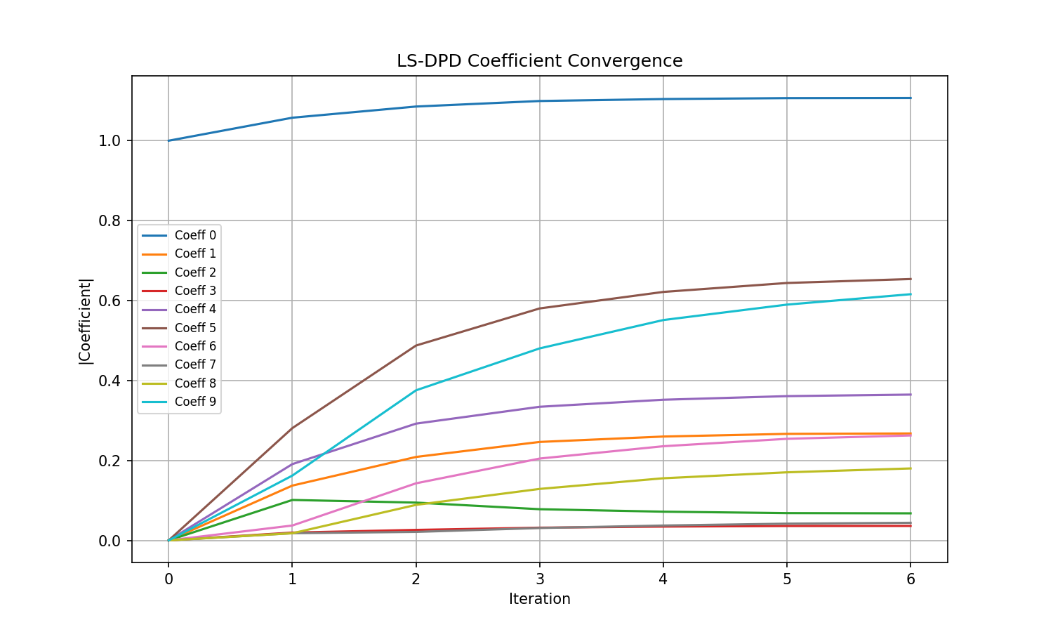
LS-DPD coefficient convergence over 6 indirect learning iterations.
The power spectral density (PSD) plot below shows a clear mitigation of out-of-band spectral emissions indicating that non-linear effects of the PA have been mostly eliminated by the DPD.
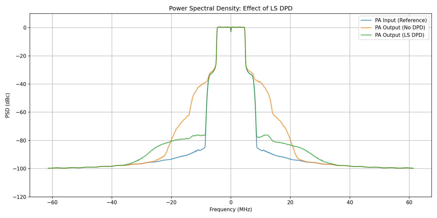
Power Spectral Density comparison: PA output without DPD, with LS-DPD, and ideal linear response.
Correspondingly, an analysis of the EVM with and without DPD reveals a clear improvement in the in-band performance.
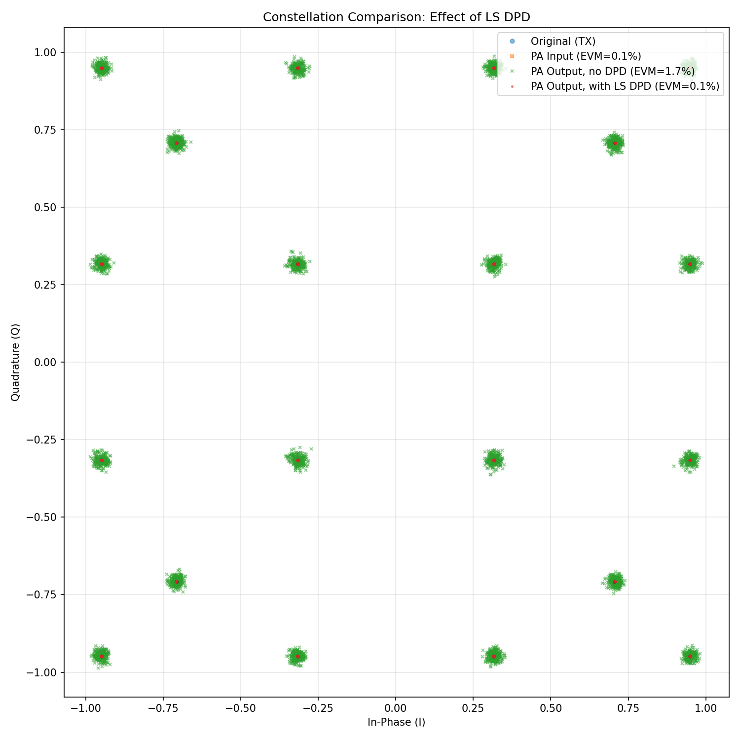
Received constellation comparison showing in-band distortion reduction with LS-DPD.
NN-DPD
After training the NN-DPD for the desired number of iterations, running inference reveals the following performance improvement.
======================================================================
NN DPD Inference
======================================================================

[1] Building evaluation system with NN DPD...
   DPD parameters:  27586
   Estimated PA gain: 0.9705 (-0.26 dB)

[2] Loading trained weights...
   Loaded weights from results/nn-dpd-weights

[3] Running inference...
   Signal shape: (16, 70144)

[4] Computing ACLR...
   ACLR (No DPD):   Lower = -35.35 dB, Upper = -34.84 dB
   ACLR (NN DPD):  Lower = -36.88 dB, Upper = -36.82 dB
   ACLR Improvement: 1.75 dB average

[5] Computing NMSE...
   NMSE (No DPD):   -22.97 dB
   NMSE (NN DPD):  -56.99 dB
   NMSE Improvement: 34.02 dB

[6] Saving PSD data...
   Saved to results/psd_data_nn.npz

[7] Saving constellation data...
   Saved to results/constellation_data_nn.npz
   EVM (PA Input):  0.07%
   EVM (No DPD):    1.65%
   EVM (NN DPD):   0.09%

======================================================================
Summary
======================================================================

Metric                             No DPD          NN DPD     Improvement
----------------------------------------------------------------------
ACLR Lower (dB)                    -35.35          -36.88            1.52
ACLR Upper (dB)                    -34.84          -36.82            1.98
NMSE (dB)                          -22.97          -56.99           34.02
EVM (%)                              1.65            0.09            1.56
----------------------------------------------------------------------
The PSD plot for NN-DPD below also shows that out-of-band spectral emissions have been suppressed, although the performance improvement in suppressing fifth-order non-linearity is smaller compared to LS-DPD.
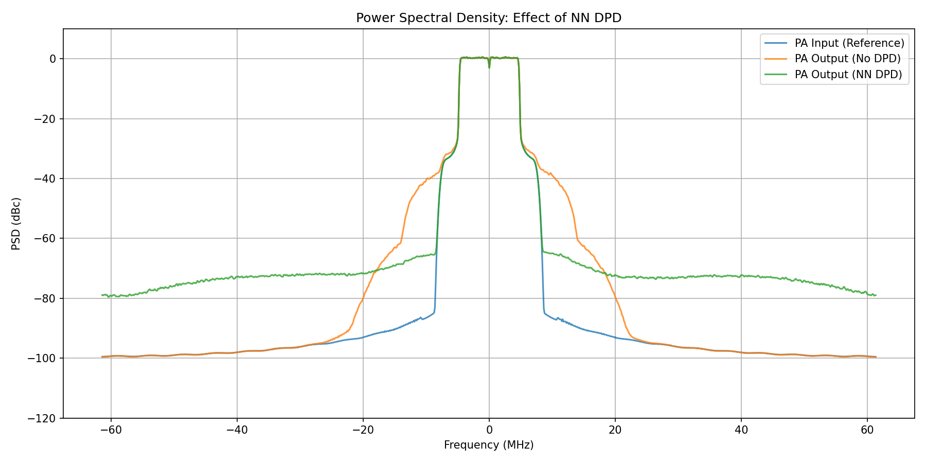
Power Spectral Density comparison: PA output without DPD, with NN-DPD, and ideal linear response.
On the other hand, the improvement in EVM with and without NN-DPD reveals a comparable improvement similar to LS-DPD.
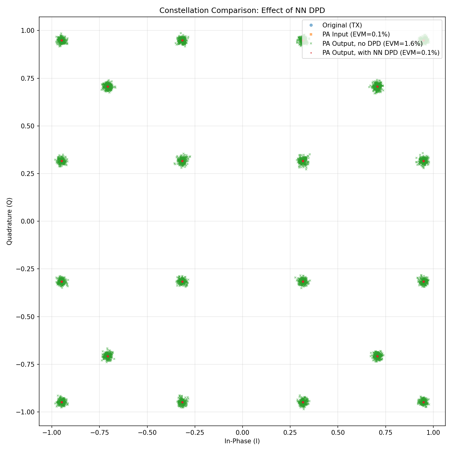
Received constellation comparison showing in-band distortion reduction with NN-DPD.
In conclusion, both DPD methods significantly reduce spectral regrowth and improve ACLR compared to the uncompensated PA output. The LS-DPD achieves faster convergence due to its closed-form solution, but such a solution might not be always feasible when the basis matrix to be inverted is ill-conditioned. Conversely, NN-DPD, due to its gradient-based learning approach is not affected by such a disadvantage and also offers flexibility for PAs with behaviors that deviate from the polynomial model.
References
[1] Dennis R. Morgan, Zhengxiang Ma, Jaehyeong Kim, Michael G. Zierdt, John Pastalan: A Generalized Memory Polynomial Model for Digital Predistortion of RF Power Amplifiers. IEEE Trans. Signal Process. 54(10): 3852-3860 (2006).
[2] Chance Tarver, Liwen Jiang, Aryan Sefidi, Joseph R. Cavallaro: Neural Network DPD via Backpropagation through a Neural Network Model of the PA. ACSSC 2019: 358-362.