MIMO-OFDM Neural Receiver
Overview
This demo implements a neural network-based receiver for MIMO-OFDM wireless communication systems using Sionna. It is a simple extension of the Neural Receiver for OFDM SIMO Systems tutorial which demonstrates a Single-Input Multiple-Output (SIMO) system, by considering a Multiple-Input Multiple-Output (MIMO)-OFDM system with 4 transmit antennas and 8 receive antennas.
The neural receiver replaces the traditional receiver chain, namely channel estimation, equalization, and demapping, with a learned convolutional neural network that directly maps received signals and noise power estimates to Log-Likelihood Ratios (LLRs) for channel decoding. This end-to-end approach allows the network to jointly optimize these operations, potentially achieving better performance than the baseline receiver, particularly under imperfect channel state information (CSI).
System Architecture
The end-to-end system (see diagram below) is architected by the System class, and the architecture diagram depicting this class is shown below.


It utilizes the configuration defined in Config to enforce a single, validated system configuration. See the code-snippet extracted from Config below for more details.
    # =========================================================================
    # Hard-coded PHY/system parameters
    # These define the physical layer configuration and should not be modified
    # without re-validating the entire simulation chain.
    # =========================================================================

    # Uplink direction: UTs transmit to BS (affects antenna role assignment)
    _direction: str = field(init=False, default="uplink", repr=False)

    # OFDM numerology: 15 kHz SCS is standard for sub-6 GHz 5G NR
    _subcarrier_spacing: float = field(init=False, default=15e3, repr=False)

    # FFT size chosen to balance frequency resolution vs. complexity
    _fft_size: int = field(init=False, default=76, repr=False)

    # 14 OFDM symbols per slot (normal cyclic prefix, 5G NR standard)
    _num_ofdm_symbols: int = field(init=False, default=14, repr=False)

    # CP length must exceed max channel delay spread to prevent ISI
    _cyclic_prefix_length: int = field(init=False, default=6, repr=False)

    # Guard carriers prevent aliasing at band edges (asymmetric for DC null)
    _num_guard_carriers: Tuple[int, int] = field(init=False, default=(5, 6), repr=False)

    # DC subcarrier nulled to avoid LO leakage issues in practical systems
    _dc_null: bool = field(init=False, default=True, repr=False)

    # Kronecker pilot pattern: orthogonal in time-frequency, good for MIMO
    _pilot_pattern: str = field(init=False, default="kronecker", repr=False)

    # Pilot positions distributed across slot for channel tracking
    _pilot_ofdm_symbol_indices: Tuple[int, ...] = field(
        init=False, default=(2, 5, 8, 11), repr=False
    )

    # 4x8 MIMO: 4 UT antennas (Tx), 8 BS antennas (Rx) for uplink
    # This asymmetry favors the BS with more receive diversity
    _num_ut_ant: int = field(init=False, default=4, repr=False)
    _num_bs_ant: int = field(init=False, default=8, repr=False)

    # QAM modulation (constellation type, not order)
    _modulation: str = field(init=False, default="qam", repr=False)

    # Default bits per symbol (overridden by user-settable num_bits_per_symbol)
    _num_bits_per_symbol: int = field(init=False, default=2, repr=False)  # QPSK

    # Rate-1/2 LDPC provides good balance of coding gain vs. complexity
    _coderate: float = field(init=False, default=0.5, repr=False)

    # Fixed seed for reproducible channel/noise realizations
    _seed: int = field(init=False, default=42, repr=False)
Tx class generates random information bits, applies LDPC encoding, maps coded bits to QPSK symbols, and places them onto an OFDM resource grid with 14 OFDM symbols per slot, a 15 kHz subcarrier spacing, and an FFT size of 76. CSI class generates the frequency-domain CDL channel for the 4x8 MIMO link with the desired delay spread, carrier frequency, mobility, and propagation scenario by first configuring dual cross-polarized transmit and receive antenna arrays according to 3GPP TR 38.901 [1], then generating delay-domain channel impulse responses (CIRs), and finally converting them into normalized frequency-domain channel coefficients consistent with the resource grid. Rx, the baseline receiver class, processes received signals by first obtaining channel estimates, then utilizing them to perform equalization, followed by demapping to produce LLRs, which are finally decoded by an LDPC decoder.
Neural Receiver
The neural receiver architecture (see diagram below), implemented in NeuralRx, is a convolutional network (as in [2]) that processes the received resource grid as a 2D image where the spatial dimensions correspond to OFDM symbols (time) and subcarriers (frequency), with channels representing the real and imaginary parts of each receive antenna plus the noise power estimate.


The architecture consists of an input convolutional layer that projects the concatenated input features to 256 feature channels, cascaded by 4 residual blocks (ResidualBlock), each built from stacking two cascaded units of layer normalization, activation function, and convolutional layer, with a skip connection to avoid gradient vanishing. The output convolutional layer produces per-subcarrier LLRs for each stream and bit position, which are then reshaped and passed through a resource-grid demapper before LDPC decoding.
The input/output layers and the residual blocks are initialized as shown below:
        # Input conv: expand from (2*num_rx_ant + 1) to num_conv2d_filters channels
        self._input_conv = Conv2D(
            filters=self.num_conv2d_filters,
            kernel_size=(3, 3),
            padding="same",
            activation=None,
        )

        # Residual stack for feature extraction
        self._res_blocks = [
            ResidualBlock(
                num_conv2d_filters=self.num_conv2d_filters,
                num_resnet_layers=self.num_resnet_layers,
            )
            for _ in range(self.num_res_blocks)
        ]

        # Output conv: contract to (num_streams x bits_per_symbol) for LLR output
        # Each output channel corresponds to one bit position in the constellation
        self._output_conv = Conv2D(
            filters=int(
                self._cfg.rg.num_streams_per_tx * self._cfg.num_bits_per_symbol
            ),
            kernel_size=(3, 3),
            padding="same",
            activation=None,
        )
and the features are processed as shown below:
        # =====================================================================
        # Neural Network Forward Pass
        # =====================================================================
        # Input convolution: expand channel dimension
        z = self._input_conv(z)

        # Residual stack: extract hierarchical features
        for block in self._res_blocks:
            z = block(z)

        # Output convolution: produce per-bit LLR predictions
        z = self._output_conv(z)
Training
Training minimizes binary cross-entropy (BCE) loss between the neural receiver’s soft LLR outputs and the transmitted coded bits, bypassing LDPC encoding/decoding for gradient flow. The training loop samples Eb/N0 uniformly from -3 dB to 7 dB for each batch, enabling the network to learn across the full SNR range simultaneously.
Gradient accumulation over 4 mini-batches of size 32 yields an effective batch size of 128, balancing memory constraints with gradient stability. The Adam optimizer with default learning rate is used. Checkpointing supports training resumption via the --iterations and --fresh command-line arguments. The core of the training logic is shown below:
# =============================================================================
# Training Step Function
# Returns loss and gradients; accumulation handled in main loop
# =============================================================================
@tf.function(
    reduce_retracing=True,
    input_signature=[
        tf.TensorSpec([], tf.int32),
        tf.TensorSpec([None], tf.float32),
    ],
)
def train_step(batch_size, ebno_vec):
    """
    Execute single forward/backward pass.

    Parameters
    ----------
    batch_size : tf.Tensor, int32, scalar
        Number of samples in batch.

    ebno_vec : tf.Tensor, float32, [batch_size]
        Per-sample Eb/N0 in dB.

    Returns
    -------
    loss : tf.Tensor, float32, scalar
        BCE loss for this batch.

    grads : List[tf.Tensor]
        Gradients for each trainable variable. None gradients are
        replaced with zeros to avoid issues in accumulation.

    Note
    ----
    The @tf.function decorator with input_signature ensures the function
    is traced once and reused, avoiding retracing overhead each iteration.
    """
    with tf.GradientTape() as tape:
        loss = system(batch_size, ebno_vec)
    grads = tape.gradient(loss, system.trainable_variables)
    # Replace None gradients with zeros (occurs for unused variables)
    grads = [
        g if g is not None else tf.zeros_like(w)
        for g, w in zip(grads, system.trainable_variables)
    ]
    return loss, grads


# =============================================================================
# Validation: Accumulation Alignment
# Start/target must align with accumulation steps for correct averaging
# =============================================================================
if start_iteration % ACCUMULATION_STEPS != 0:
    raise ValueError("start_iteration must be a multiple of ACCUMULATION_STEPS")

if target_iteration % ACCUMULATION_STEPS != 0:
    raise ValueError("target_iteration must be a multiple of ACCUMULATION_STEPS")

# =============================================================================
# Training Loop
# Gradient accumulation: sum gradients over ACCUMULATION_STEPS, then apply
# =============================================================================
accumulated_grads = None
for i in range(start_iteration, target_iteration):
    # Sample random Eb/N0 for each batch element
    # Training across SNR range improves generalization
    ebno_db = rng.uniform([BATCH_SIZE], EBN0_DB_MIN, EBN0_DB_MAX, tf.float32)
    loss, grads = train_step(tf.constant(BATCH_SIZE, tf.int32), ebno_db)

    # Accumulate gradients
    if accumulated_grads is None:
        accumulated_grads = [tf.Variable(g, trainable=False) for g in grads]
    else:
        for acc_g, g in zip(accumulated_grads, grads):
            acc_g.assign_add(g)

    # Apply accumulated gradients every ACCUMULATION_STEPS iterations
    if (i + 1) % ACCUMULATION_STEPS == 0:
        avg_grads = [g / ACCUMULATION_STEPS for g in accumulated_grads]
        optimizer.apply_gradients(zip(avg_grads, system.trainable_variables))
        accumulated_grads = None

    loss_value = float(loss.numpy())
    loss_history.append(loss_value)

    print(
        f"\rStep {i}/{target_iteration}  Loss: {loss_value:.4f}",
        end="",
        flush=True,
    )
print("\n\nTraining complete.")
Results
Performance is evaluated using Bit Error Rate (BER) and Block Error Rate (BLER) across Eb/N0 from -3 dB to 6 dB under the CDL-C channel model. The baseline receiver uses LS channel estimation with LMMSE equalization, tested under both perfect CSI and imperfect CSI (estimated channel) conditions.
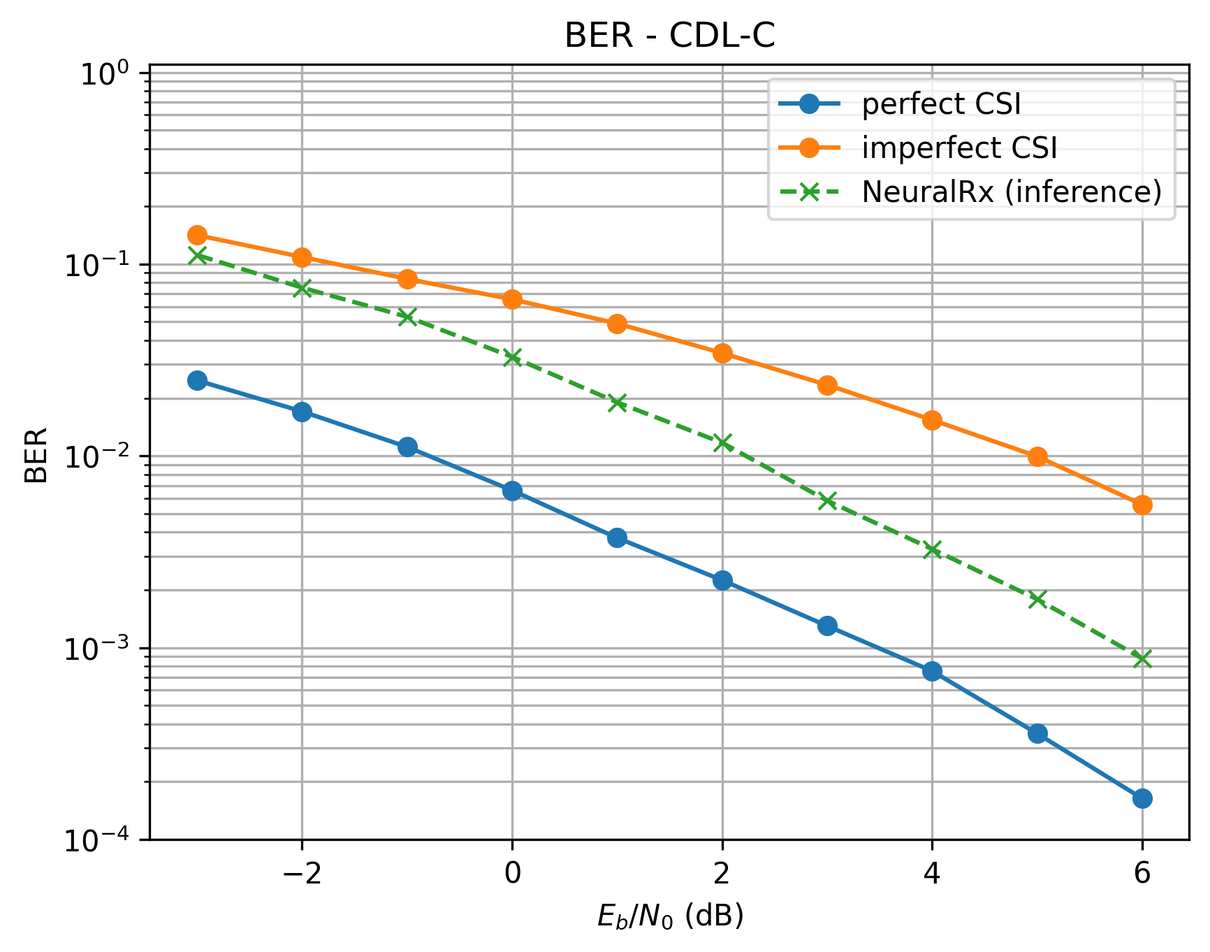
BER comparison under CDL-C channel: neural receiver vs. baseline with perfect/imperfect CSI.
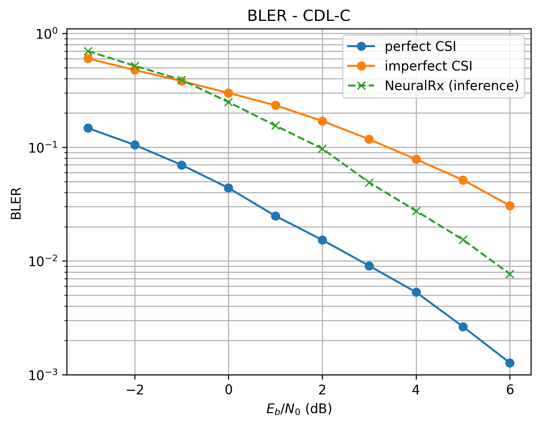
BLER comparison under CDL-C channel: neural receiver vs. baseline with perfect/imperfect CSI.
The neural receiver significantly outperforms the baseline with imperfect CSI, particularly at mid-to-high SNR where channel estimation errors dominate baseline performance. At 6 dB Eb/N0, the neural receiver achieves approximately 4x lower BER than the imperfect-CSI baseline. However, the neural receiver does not yet match the perfect-CSI baseline, indicating room for architectural improvements or increased model capacity.
References
[1] 3GPP TR 38.901, “Study on channel model for frequencies from 0.5 to 100 GHz”, Release 18.0.
[2] M. Honkala, D. Korpi and J. M. J. Huttunen, “DeepRx: Fully Convolutional Deep Learning Receiver,” in IEEE Transactions on Wireless Communications, vol. 20, no. 6, pp. 3925-3940, June 2021, doi: 10.1109/TWC.2021.3054520.